
A CFD surrogate model answers in milliseconds what a solver answers in minutes: the full velocity, pressure, and temperature fields at any parameter values inside a trained range. CFD AI builds these surrogates from your COMSOL simulations using physics-informed neural networks — behind a desktop GUI, no PyTorch knowledge required.
What is a physics-informed neural network?
A neural network trained on two signals at once: your COMSOL solutions (supervised data) and the governing equations themselves — Navier–Stokes and energy conservation — enforced as residual penalties. The physics term buys physical consistency and robustness on sparse data; your solver’s data does the heavy lifting. The result maps (x, y, z, time, parameters) → (u, v, w, p, T) continuously, so one trained network replaces an entire parametric sweep. Deeper dive: PINNs explained — when can AI replace CFD?
Which physics does it detect?
- Flow: incompressible laminar and turbulent (k-ε, k-ω, SST, L-VEL, Spalart–Allmaras, Realizable k-ε detected automatically)
- Heat transfer: advection–diffusion, conjugate heat transfer, multi-body models with any number of solids and fluids — property jumps carried exactly per body
- Geometry: 2D planar, 2D axisymmetric (full cylindrical residuals), and true 3D on the real COMSOL mesh
- Time: steady or transient — time steps are sampled automatically and the unsteady terms join the training constraints
- Boundary conditions: all of them — learned from the data, so no BC type limits the surrogate; material properties are imported from the model automatically
The four-step workflow
- Generate data — load the .mph, pick the parameters to learn over; CFD AI suggests how many runs you need, samples them by Latin Hypercube, and runs COMSOL for you.
- Train — pick from 8 architectures (MLP, Modified MLP, Fourier features, SIREN, DeepONet, Mesh GNN, MeshGraphNet, PIPN; the best is auto-suggested — graph networks even learn across geometry-changing parameters) with live loss curves, validation, and best-epoch restore. A GPU edition bundles CUDA PyTorch.
- Explore — contours, COMSOL-style 3D views with cut planes on the true mesh, slices, probes, sweeps, animations — all from the surrogate, no COMSOL license in the loop.
- Optimize & export — 16 optimization methods over the trained model; a Simulink-style canvas chains surrogates into whole-system models; export to Python, MATLAB, dependency-free C++17, Simulink, or a self-contained interactive HTML page.
The eight network architectures
Training a good surrogate is an architecture decision, and no single network wins everywhere — which is why CFD AI ships eight and suggests the best one automatically from your model’s physics, geometry, and parameters. Coordinate networks (MLP, Modified MLP, Fourier, SIREN) excel on smooth fields and sharp gradients; operator and graph networks (DeepONet, Mesh GNN, MeshGraphNet, PIPN) learn on the mesh itself and generalize across geometry-changing parameters.
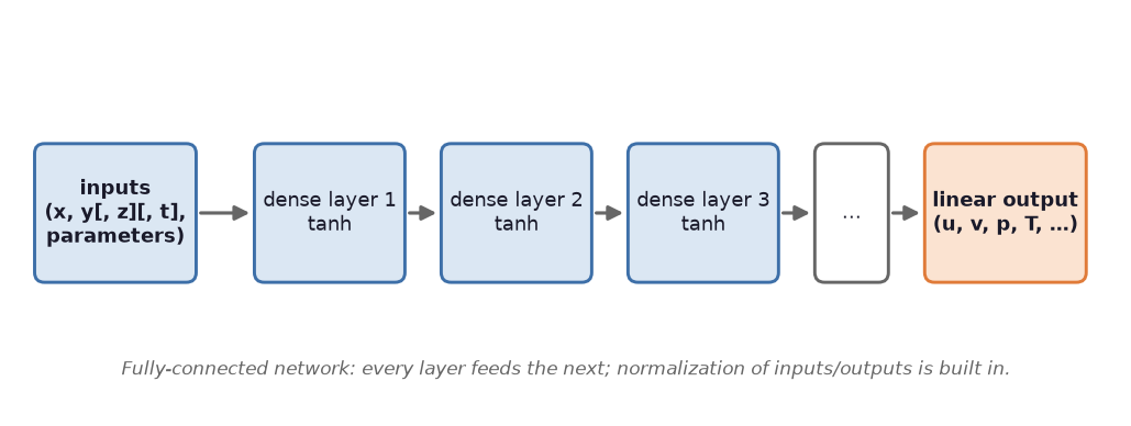
MLP
The classic physics-informed network: coordinates and parameters in, fields out through fully-connected layers. Fast to train and hard to beat on smooth, steady flows.
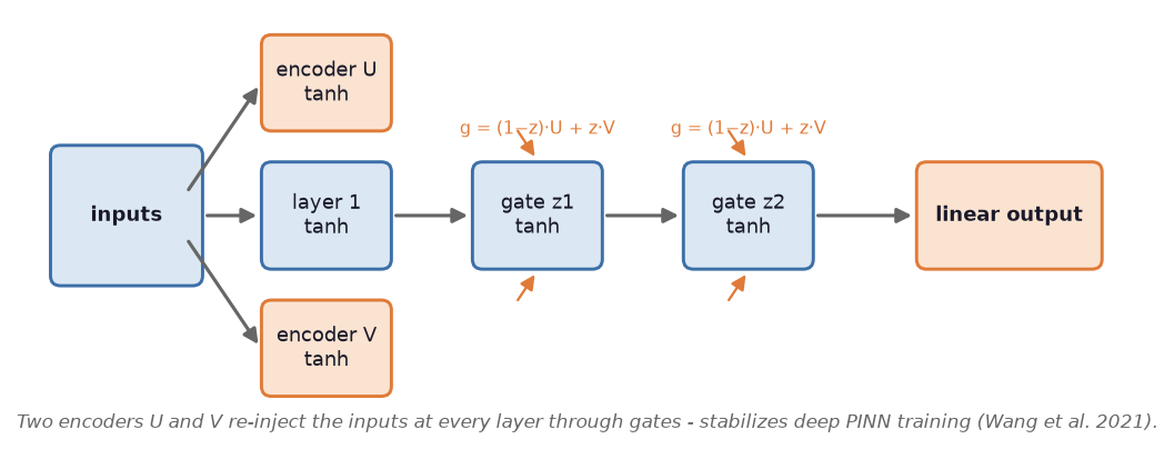
Modified MLP
Adds gated skip connections that cure the gradient pathologies PINNs are known for — noticeably better on stiff, multi-scale problems.
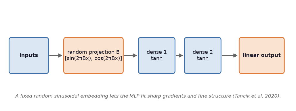
Fourier features
Projects the inputs through random sinusoids before the network, defeating spectral bias so fine vortices and thin boundary layers are actually learned.
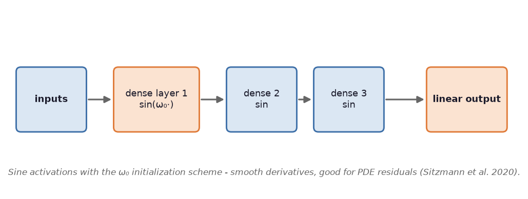
SIREN
Sinusoidal activations throughout — represents sharp gradients and periodic structure with striking precision.
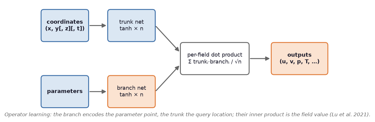
DeepONet
A branch–trunk operator network that learns the mapping from parameters to whole solution fields — excellent generalization across operating points.
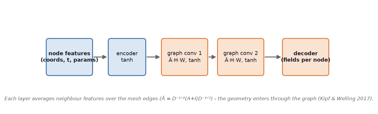
Mesh GNN
Message passing directly on the COMSOL mesh graph. Because it learns on geometry, it generalizes across geometry-changing parameters — something coordinate networks cannot do.
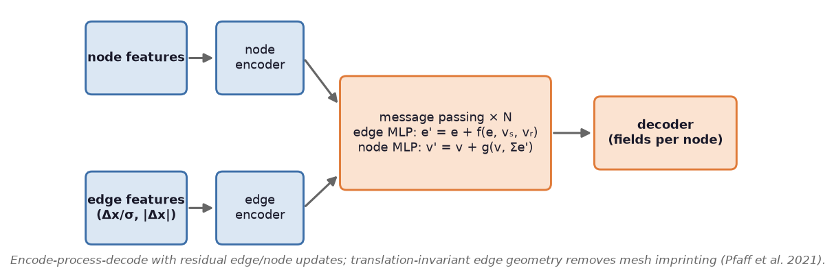
MeshGraphNet
The simulation-grade graph network: deeper message passing with edge features, built for complex unstructured meshes.
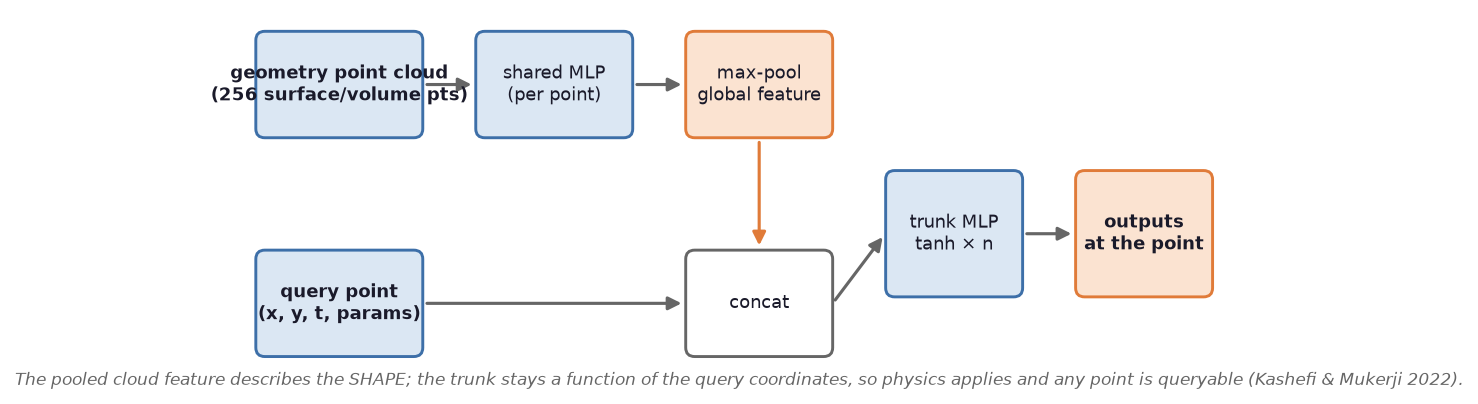
PIPN
A physics-informed point network operating on point clouds — geometry-flexible without needing mesh connectivity at all.

How accurate is a trained surrogate?
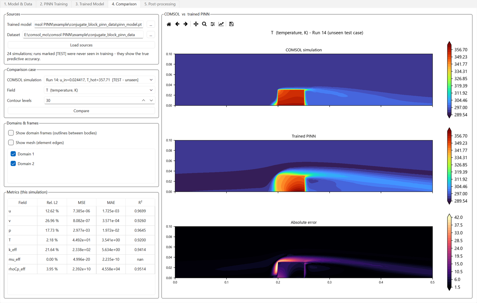
Measured on held-out test simulations, not marketing copy: a turbulent backward-facing step (k-ε RANS, Re ≈ 50,000) reaches ~1–2% relative error on velocity and 0.02% on temperature; a conjugate heat-transfer case learns an effective-conductivity field across a 267× property jump at R² = 0.94; a full-3D shell-and-tube heat exchanger reaches ≈2.4% temperature error from 14 solves of an 8-minute RANS model. Every example ships with its dataset and checkpoint so you can reproduce the numbers, and any prediction can be verified against a fresh COMSOL solve at that exact operating point.
Common questions
Do I need COMSOL on the machine that uses the surrogate?
No. COMSOL is needed only to generate training data and for optional verification solves. Training, exploring, optimizing, the system canvas, and all five exports run from the dataset and checkpoint alone.
Can the exported model run outside the app?
Yes — five ways: a Python module, plain MATLAB (no toolboxes), a dependency-free C++17 project, a Simulink block, and an interactive HTML page that runs entirely in a browser. Each export includes a built-in self-test against reference values.
GPU or CPU?
Both editions exist. The GPU edition bundles CUDA PyTorch for fast training on NVIDIA cards; the CPU edition trains fine for smaller models. Checkpoints are interchangeable between editions.
Try CFD AI on your own model — free
Download the demo and see the workflow for yourself, or take a free 2-day trial license of the full edition — activated in minutes, no credit card charged. A GPU edition (CUDA) is available on the product page.