
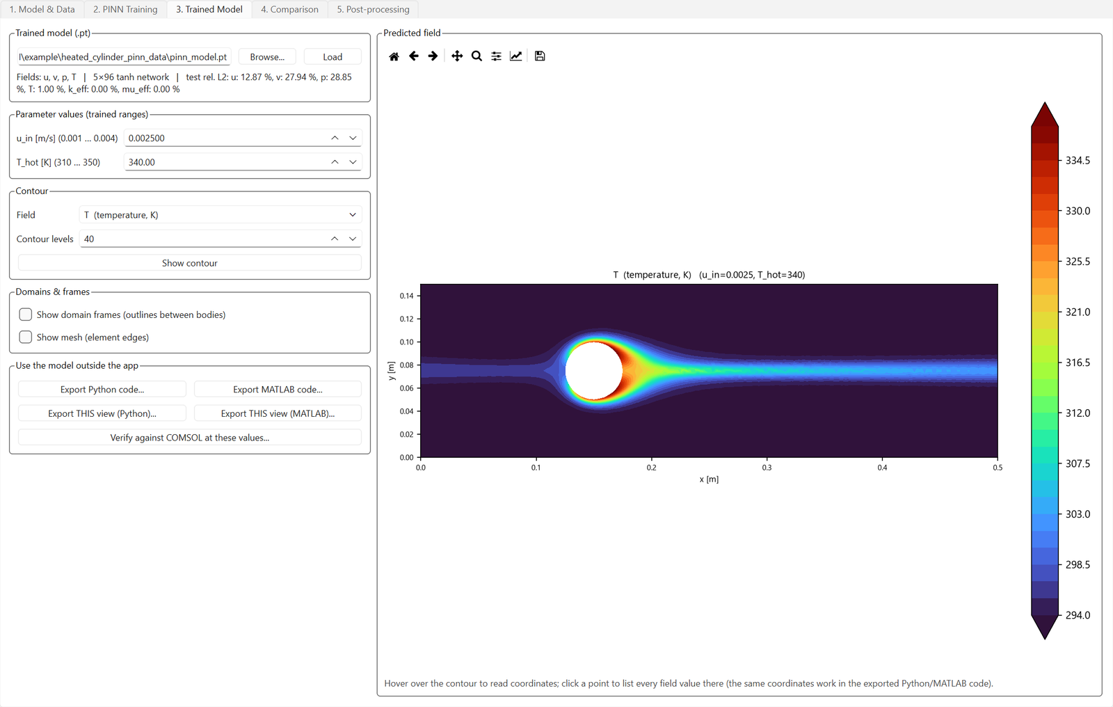
A physics-informed neural network (PINN) is a neural network trained to reproduce simulation fields — velocity, pressure, temperature — while being penalized whenever its predictions violate the governing equations. The result is a surrogate model: once trained on a set of CFD solutions, it predicts the full field at new parameter values in milliseconds instead of minutes.
What exactly does the “physics” part add?
During training, the network’s outputs are differentiated and substituted into the PDEs (Navier–Stokes, energy conservation); the residual becomes an extra loss term alongside the data-fitting loss. Measured honestly, the physics loss is not a magic accuracy boost — on well-sampled problems it mainly buys physical consistency, robustness to sparse or noisy data, and physically meaningful learned fields (like effective viscosity in turbulent flows). Data from your solver still does the heavy lifting.
When is a PINN surrogate the right tool?
- Design exploration — sweep a parameter across its range in under a second instead of queuing a parametric study
- Optimization — evolutionary algorithms need thousands of evaluations; a surrogate makes that free
- Embedding — export the trained model to Python, MATLAB, Simulink, C++, or a browser page and use it inside a bigger system model
- What-if reviews — answer “what if the inlet runs 10% hotter?” live in a meeting
When is it the wrong tool?
A surrogate approximates a family of solutions that differ only in their parameters — it does not replace the solver for new geometries or physics outside the trained range, and extrapolation beyond trained bounds is untrustworthy by construction. If you need one high-fidelity answer to one configuration, just run the solver.
How accurate can this get on real problems?
Numbers from held-out test cases in CFD AI‘s bundled examples: a turbulent backward-facing step (k-ε RANS, Re ≈ 50,000) reaches ~1–2% relative error on velocity and 0.02% on temperature; a conjugate heat-transfer case learns the effective conductivity field across a 267× property jump at R² = 0.94; and a full-3D shell-and-tube heat exchanger reaches ≈2.4% temperature error trained on just 14 solves of an 8-minute RANS model. Each prediction can also be verified against a fresh COMSOL solve at the exact operating point — the honest way to trust a surrogate.
Do you need to know PyTorch?
No. Tools like CFD AI wrap the whole workflow — sampling the training runs with Latin Hypercube, choosing among eight network architectures, training with validation and best-epoch restore, and reporting per-field error metrics — behind a desktop GUI. Machine-learning literacy helps you interpret results; it is no longer the price of admission.