
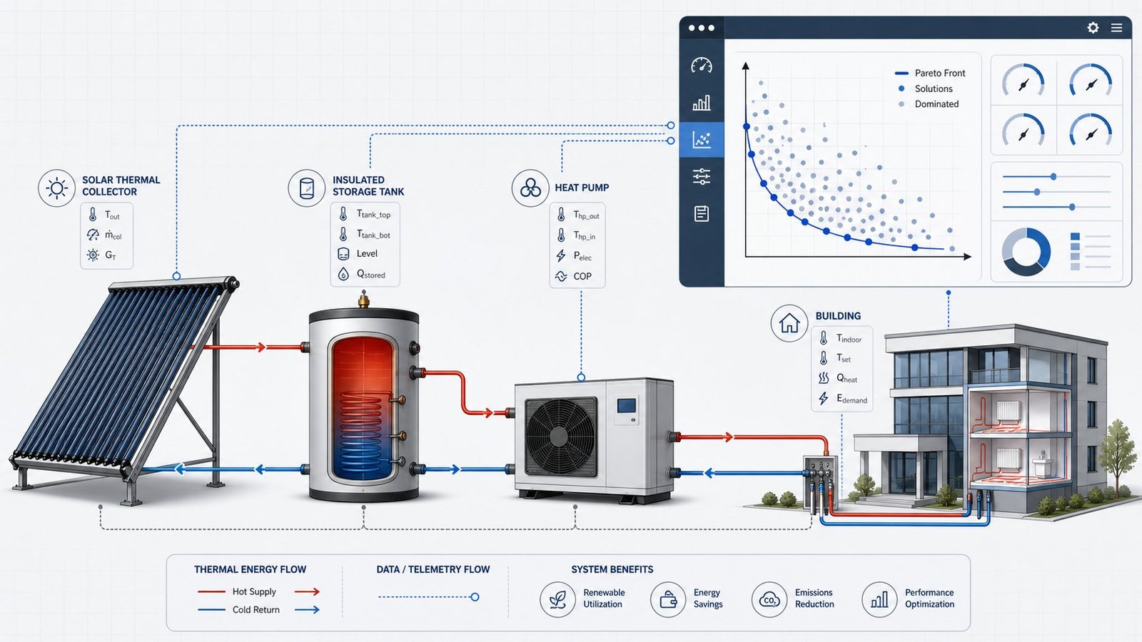
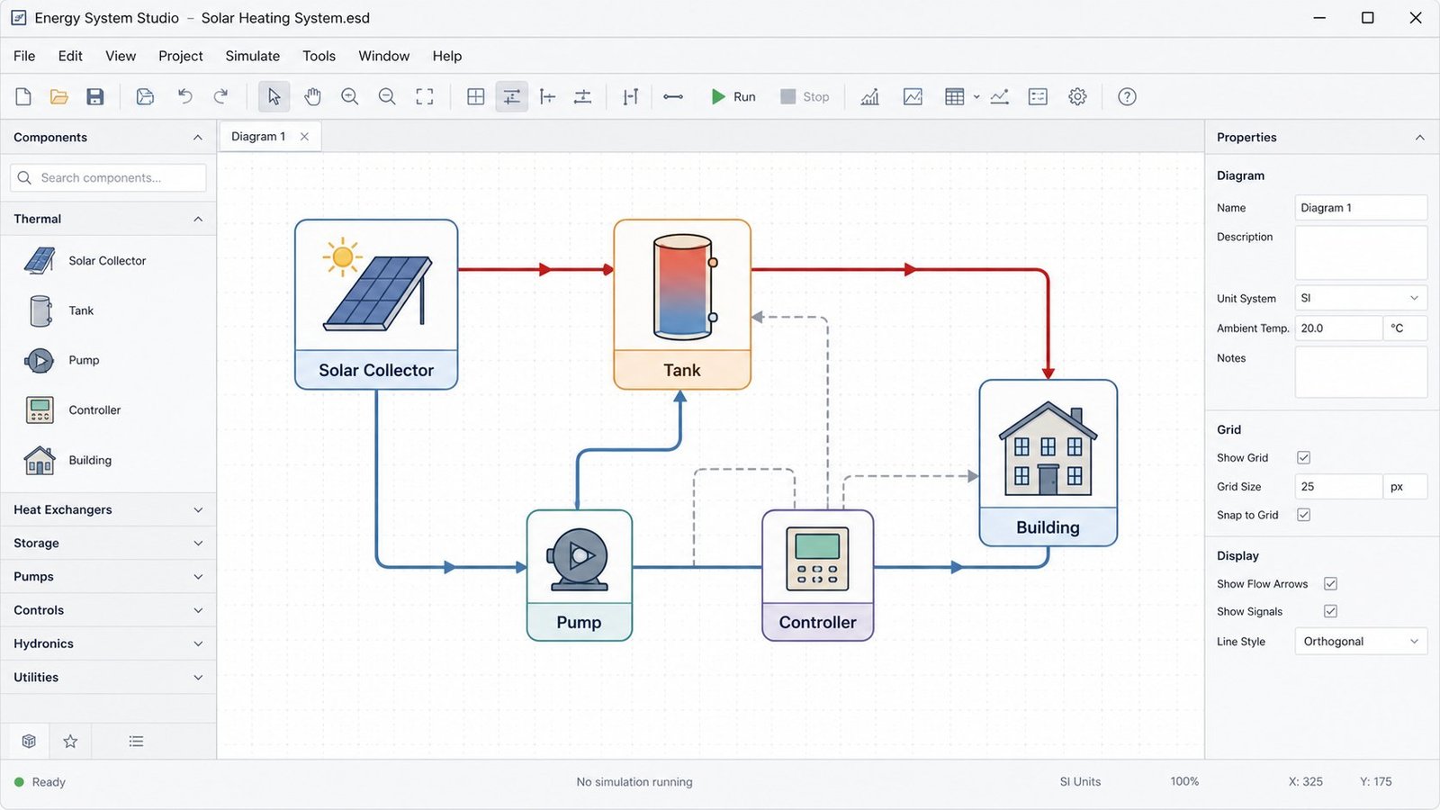
TRNSYS is a transient systems simulation program used for energy system modeling — solar thermal plants, ground-source heat pump loops, district heating networks, and whole-building energy models. You connect components — a collector, a storage tank, a pump, a controller — into a deck, then run it against a full year of weather data at time steps as short as one minute.
Most engineers stop at a working model. The next step — finding the design that minimizes cost, energy use, and pump work at the same time — is where the built-in tools run out. A typical deck carries 8-20 free variables: collector area, tank volume, flow rate, setpoint temperatures. Testing combinations by hand in the Simulation Studio takes days. Our optimization module couples directly to your input file (.dck) and runs hundreds of simulations in parallel across your available CPU cores.
What TRNSYS Does for Energy System Simulation
The name stands for Transient System Simulation. It was built at the University of Wisconsin for detailed, time-resolved energy modeling. Each component in a deck is a Type: Type56 for a multi-zone building, Type534 for a borehole field, Type1 for a flat-plate solar collector. You wire Types together, feed in a TMY3 weather file, and the solver marches through 8,760 hours computing temperatures, flow rates, and loads at every point in the system. That level of detail is why the tool is standard in solar thermal design, geothermal sizing, CHP dispatch studies, and building energy code compliance work.
Common Applications
Engineers reach for this platform whenever hour-by-hour or sub-hourly behavior matters more than an annual average. A solar combi-system needs to know how storage temperature drifts over a cold week, not just its yearly solar fraction. A datacenter cooling loop needs to know how a chiller responds to a load spike, not just its design-day capacity.
- Solar thermal and PVT systems — collector field sizing, storage stratification, backup heater control
- Ground-source and air-source heat pump loops — borehole length, buffer tank volume, defrost cycling
- District heating and cooling networks — pipe losses, pump scheduling, substation control logic
- Building energy code compliance and retrofit studies — envelope, HVAC, and controls interaction
Where a Standalone Model Hits Its Limits
A single run tells you how one design performs. It does not tell you which design is best. Once you balance more than one objective — lower levelized cost against lower CO2 against higher solar fraction — manual iteration stops scaling. A detailed building-plus-plant deck can take 3-10 minutes per run; testing 500 combinations sequentially means over 50 hours of compute before you’ve even compared results. Most teams settle for a handful of manually chosen cases instead of an actual search of the design space.
Coupling Multi Optimization to Your Deck
Our module reads your existing .dck file, exposes the variables you flag — collector area, tank volume, mass flow rate, control setpoints — and drives a genetic algorithm (NSGA-II by default) across a population of 40-100 candidate designs per generation. Instead of one run at a time, it launches batches in parallel across your available cores, so a 10-minute deck evaluated 600 times finishes in hours, not days. The result is a Pareto front: a set of designs where improving cost means giving up performance elsewhere, and you pick the trade-off that fits your project. The same engine also drives EES and COMSOL models, so a mixed workflow — say, a system deck plus a COMSOL heat exchanger — optimizes as one problem.
FAQ
How many objectives can the optimizer handle at once?
Two to four in practice. Beyond four, the Pareto front becomes hard to visualize and interpret, though the algorithm itself can technically run more.
Do I need to rebuild my deck to use the optimization module?
No. You keep your existing components and connections. You flag which parameters vary and which outputs matter, and the module handles the run scheduling.
How long does a typical optimization take?
For a deck that runs in 3-5 minutes, expect a few hours across 40 CPU cores for 500-800 evaluations — enough for the genetic algorithm to converge on a stable front.
Get Your Model Optimized
If your deck already runs and you’re ready to search the design space instead of guessing at it, visit TRNSYS Optimization for setup details and typical run counts, or reach out through Contact Us to discuss your specific model.