
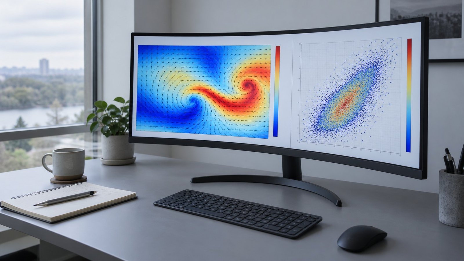
Your PINN reached a training loss of 3e-6 and the velocity field is still wrong. The optimizer is fine. Why PINNs fail CFD reduces to one sentence from Andersen & Matsubara in PINNs Failure Modes are Overfitting (arXiv:2605.30910, submitted 29 May 2026): the loss is minimized on the collocation points, but not elsewhere. Your network learned the sample set, not the PDE.
This is a debugging manual, not an introduction. We skip what a PINN is and whether it replaces a solver — our earlier posts cover both. Here you get five named failure modes, the diagnostic for each, and the collocation and weighting settings we now ship on client CFD surrogates.
Why PINNs Fail CFD at a Loss of 1e-6
Treat the residual like a test set. The collocation points PINN training samples are not scenery — they are the only place the physics is enforced. Evaluate the same residual on an independent grid four times denser and the number usually jumps one to three orders of magnitude. That gap is the failure. Andersen & Matsubara show that regularization plus double backpropagation across all residual terms matched the best published results on four standard failure-mode equations while using up to 23× fewer collocation points.
So stop adding points. Start looking at where the residual lives.

Five PINN Training Failure Modes You Can Diagnose in an Afternoon
Most PINN convergence problems clients send us collapse into five patterns. Each has a symptom you already saw, a diagnostic that takes under 20 minutes, and a fix.
1. Collocation-point overfitting
Symptom: loss curve is textbook, the field is not. Diagnostic: resample 4× denser and re-evaluate the residual without training; plot it as a map. Fix: residual-based adaptive resampling every 2,000 iterations, plus a gradient penalty on the residual — double backpropagation. On a 2D backward-facing step we cut 60,000 interior points to 12,000 and the held-out residual dropped by 8×.
2. Loss-term imbalance between PDE, BC and IC
Symptom: momentum satisfied, wall slips by 4 percent of inlet velocity. Or the boundary is exact and the core is smeared. Diagnostic: log each term and its gradient norm at the last hidden layer, per epoch. If the PDE gradient is 100× the BC gradient, weighting is the problem, not capacity. Fix: gradient-norm annealing updated every 100 steps.
3. Spectral bias on vortex-dominated fields
Symptom: the recirculation bubble is missing and the shear layer is diffused. Diagnostic: take a line probe across the wake and FFT it against reference data; energy above wavenumber 8 will be near zero. Fix: Fourier feature embedding with a spread of scales, or split the domain — we use 4 to 9 subdomains on lid-driven cavity at Re = 2,000.
4. Causality violation in transient runs
Symptom: t = 10 s looks plausible, t = 0.5 s is nonsense, and vortex shedding starts at the wrong phase. Diagnostic: plot residual against time. If early time is no better than late time, the network optimized the whole horizon at once. Fix: causal weighting, or march in windows of 20 to 40 time steps with the previous window frozen.
5. Collapse to a trivial solution on stiff PDEs
Symptom: the field goes near-uniform, loss falls monotonically, and convection dominates. Diagnostic: compare the predicted field standard deviation to the boundary range — under 5 percent means collapse. Fix: hard-constrain boundaries through an ansatz so they cannot be traded away, then ramp Reynolds or Peclet number over the first 30 percent of training.
The Collocation and Weighting Settings We Ship
Our PINN loss balancing CFD recipe is three numbers and one schedule. Start at weights of 1 for the PDE residual and 100 for boundary and initial residuals. Hand control to gradient-norm balancing after 5,000 iterations. Sample 10,000 to 15,000 interior points, 2,000 boundary points, resample adaptively. Keep 20 percent of points as a frozen residual test set you never train on — that single habit catches mode 1 before a client ever sees the surrogate.
We reserve residual maps as the primary review artifact. A loss curve hides the failure; a map of where the equation is violated shows it in one glance.
Sweeping weights in parallel instead of guessing
One run at a time is how weeks disappear. We sweep loss weights, Fourier scales, depth and width as a parallel study across 32 to 64 cores — the same execution model behind our AI and machine learning simulation tools. A 96-configuration sweep that runs 41 hours serially finishes in about 55 minutes. Reference fields come from COMSOL runs driven through our optimizer, so the validation data is generated the same way every time.

Where PINNs Earn Their Place, and Where They Do Not
Be honest about scope. The June 2025 survey Physics-Informed Neural Networks for Industrial Gas Turbines (arXiv:2506.19503) describes PINN use in turbomachinery as still in its early stages, needing refinement and standardization before it carries production decisions. Treat that as a constraint on your claims, not a reason to stop.
The June 2026 review Beyond Data-Driven (arXiv:2606.21945) points to the regimes where PINNs genuinely win: sparse-data problems, inverse problems such as recovering an unknown boundary flux, and differentiable design workflows where you need gradients through the model. Those are the jobs we accept. A 30-million-cell production RANS run is not one of them.
Pre-Flight Checklist Before You Trust a Flow Field
- Evaluate the residual on a 4× denser independent grid. Report both numbers, never just the training loss.
- Render a residual map per equation term. Look for structure, not magnitude.
- Log PDE, BC and IC losses separately with their gradient norms.
- FFT a line probe against reference data and check energy above wavenumber 8.
- Plot residual against time for any transient case.
- Compare field standard deviation to boundary range; below 5 percent, suspect collapse.
- Repeat the run with 3 seeds. Spread above 10 percent in integral quantities means the setup, not the seed, is unstable.
FAQ
Does adding more collocation points fix the problem?
Usually not. Andersen & Matsubara reached comparable accuracy with up to 23× fewer points by regularizing the residual instead. Denser sampling raises cost and often leaves the same structured error between points.
How do I tell overfitting from spectral bias?
Look at the residual map. Overfitting shows speckle between sample locations. Spectral bias shows smooth, broad error concentrated in shear layers and vortex cores, with high-wavenumber energy missing from the FFT.
Should I add labeled CFD data to a failing PINN?
A few hundred labeled points break trivial-solution collapse quickly. But if the residual test gap is large, data hides the symptom rather than fixing the model. Repair the sampling and weighting first.
Start From a Working Setup
Run the checklist before you argue with the architecture. Five failure modes, one residual map each, and most cases resolve in a day. If you would rather not rebuild the tooling, our AI CFD surrogate modeling service ships these diagnostics, the parallel weight sweep and the validated settings as a package. Send us the geometry and the boundary conditions through our contact page and we will tell you whether a PINN suits the case — or whether it does not.