
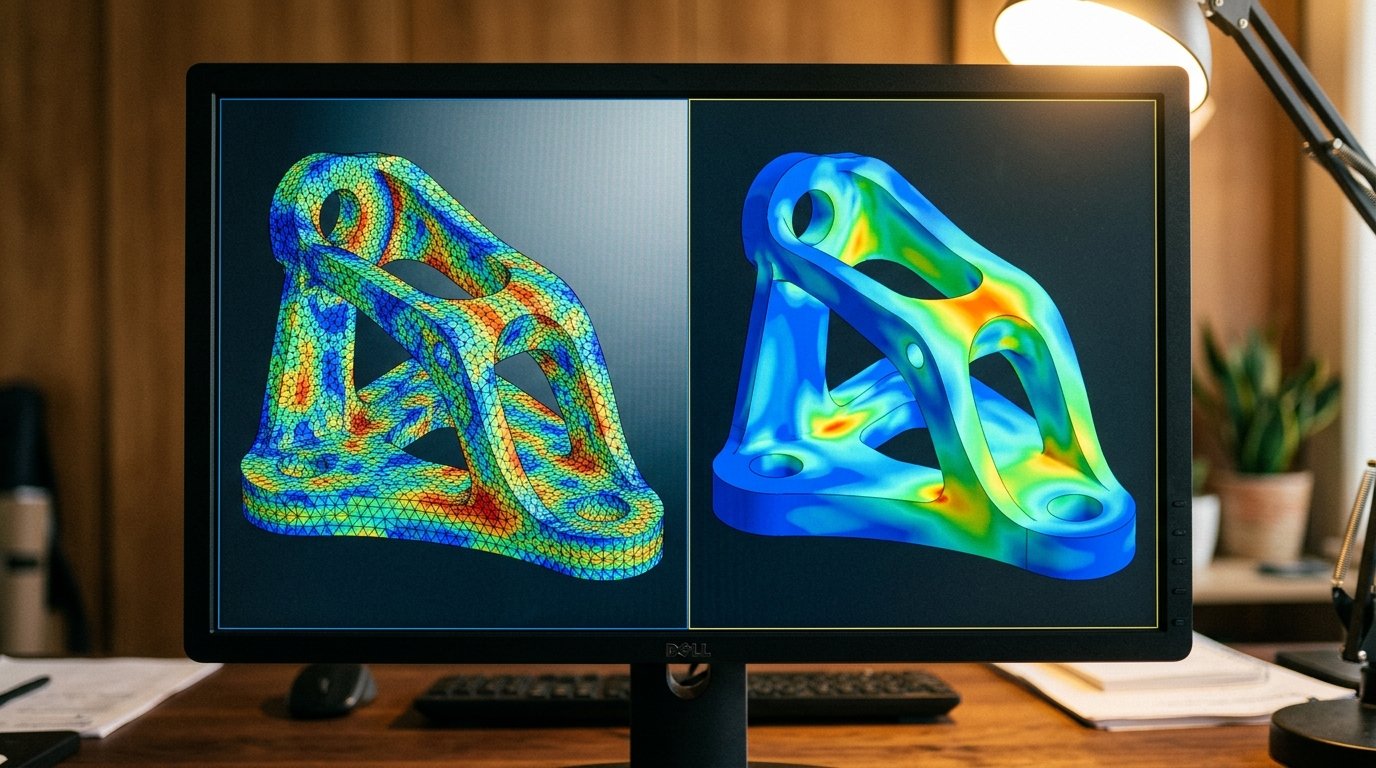
COMSOL 6.2 ships a comsol ai surrogate model workflow directly inside Multiphysics, no external Python pipeline required. The release adds a Deep Neural Network (DNN) surrogate to the base package, plus Gaussian Process (GP) and Polynomial Chaos Expansion (PCE) models for anyone holding the Uncertainty Quantification Module. All three train against a new Surrogate Model Training study built around Latin Hypercube Sampling, per COMSOL’s own 6.2 release notes.
That’s a real change for anyone running parametric sweeps in COMSOL — but it raises a question we hear from clients every week: stick with COMSOL’s native surrogate, or build a physics-informed neural network (PINN) instead? This post covers what comsol 6.2 surrogate models actually do, where the native tool runs out of road, and how we wire either option into a parallel multi-objective search across TRNSYS, EES and COMSOL projects.
Inside the COMSOL AI Surrogate Model Workflow
The Surrogate Model Training study replaces manual design-of-experiments scripting. You define input ranges, COMSOL samples them with Latin Hypercube Sampling, and the study runs your full model at each sample point to build a training set. LHS spreads points across the input space more efficiently than random or grid sampling, which is why COMSOL adopted it as the default for this study. That makes the Surrogate Model Training study a genuine comsol optimization tool, not just a curve-fitting utility — the same trained function can feed an optimization loop directly.
Simulation counts for comsol 6.2 surrogate models scale with model complexity. A simple, well-behaved case — a single nonlinear battery curve, for example — can train on as few as 20 to 30 simulations. A coupled multiphysics model, such as a thermally actuated MEMS device with electromagnetics, heat transfer and structural mechanics running together, can need thousands of raw simulations before the surrogate tracks the full model closely. Training itself is comparatively cheap: COMSOL reports a few hours on a desktop workstation or a few minutes on a cluster, once the data set exists.
- DNN (Deep Neural Network) — included in base COMSOL Multiphysics; handles the largest data sets but returns no uncertainty estimate.
- Gaussian Process (GP) — requires the Uncertainty Quantification Module; returns a confidence band around each prediction.
- Polynomial Chaos Expansion (PCE) — also requires the Uncertainty Quantification Module; strongest on smooth, lower-dimensional responses with uncertainty bands.

The Interpolation Trap: Why You Can’t Extrapolate
Every one of these models is fit to the envelope you sampled — nothing more. Engineering.com’s interview with COMSOL’s Björn Sjödin makes this explicit: surrogate models are well suited to interpolation inside the trained parameter range, but they should not be used to extrapolate beyond it. Push an input past the bounds of your Latin Hypercube sample and the surrogate keeps returning a number — it just stops being a trustworthy one.
In practice, this means you size your design-of-experiments bounds around the real range your optimization run will explore, not the range you think might be interesting someday. If a downstream NSGA-style search proposes a design outside the trained envelope, the surrogate call still returns instantly, but the result is unverified. We flag that risk to clients before we wire any surrogate — native or PINN — into an automated search loop.
See also: Why PINNs Fail CFD: A Field Debugging Guide
PINN vs COMSOL Surrogate: Picking the Right Tool
The PINN vs COMSOL surrogate decision comes down to how your design space is built, not which technology sounds more advanced. COMSOL’s native surrogate needs a finished design-of-experiments sweep before it can train — you run the samples, then fit DNN, GP or PCE on top. A PINN skips that step. It trains directly against the governing equations and boundary conditions, so there’s no pre-run sweep to size or wait on.
That flexibility comes with a cost. A PINN needs someone who can tune the physics-loss weighting, balance data loss against PDE residual loss, and diagnose why a network satisfies the boundary conditions but drifts on the interior. COMSOL’s point-and-click surrogate needs none of that — you pick DNN, GP or PCE from a list and let the Surrogate Model Training study handle the rest.
- Single-physics parametric sweep, small and well-bounded design space: use COMSOL’s native surrogate. Native comsol optimization algorithms — the gradient-based and genetic solvers in the Optimization Module — can call the resulting function directly.
- Large or multi-solver design space — COMSOL coupled with TRNSYS or EES models, or a geometry family that spans multiple trained envelopes: a purpose-built PINN or hybrid model is worth the extra setup time.
- Need an uncertainty band on the prediction itself, not just a point estimate: use GP or PCE, not DNN — DNN gives you speed and capacity, not confidence intervals.
See also: surrogate modelling cfd
Wiring a Surrogate Into a Parallel Multi-Objective Search
Multi Optimization’s AI surrogate platform treats a COMSOL surrogate — native DNN/GP/PCE or a custom PINN — as one objective evaluator inside a parallel NSGA-style search. The surrogate function sits where a full COMSOL solve used to sit in the evaluation loop. Population size, crossover and Pareto ranking run exactly as they would against the full model, just against a function call instead of a finite element solve.
The payoff shows up in wall-clock time. In one client comparison we ran, a single COMSOL evaluation took 14 minutes per design point on the full multiphysics model. After we substituted a trained DNN surrogate for that objective, the same evaluation returned in under half a second. An 8-objective NSGA-III search that needed roughly 40,000 evaluations to converge finished in under 3 hours on a 32-core node — a run that would have taken well over a year of continuous solving against the full model.
That comparison also showed the limits described above. Two candidate designs near the edge of the sampled parameter envelope came back with surrogate predictions that disagreed with a full COMSOL re-solve by more than 12%. We now re-verify any Pareto-front candidate near the sampling boundary against the full model before it goes into a client report — the surrogate accelerates the search, it doesn’t replace final verification.

FAQ
Does COMSOL 6.2 surrogate modeling replace a PINN?
No. It replaces the need to build your own DNN pipeline for simple, single-physics sweeps. For multi-solver design spaces or geometries that fall outside a trained envelope, a PINN or hybrid model still does a job COMSOL’s native surrogate wasn’t built for.
How many simulations does a comsol ai surrogate model need to train?
As few as 20 to 30 for a simple, well-bounded case, according to COMSOL’s 6.2 release notes. Complex coupled multiphysics models can need thousands of raw simulations before the surrogate holds up across the full input range.
Can I use a COMSOL surrogate outside the range I trained it on?
No. COMSOL’s own guidance, echoed in Engineering.com’s coverage of the 6.2 release, is that these models interpolate well but shouldn’t be used to extrapolate. Keep your optimization bounds inside the trained envelope.
Does Multi Optimization support COMSOL’s native surrogate models?
Yes. We wrap a trained DNN, GP or PCE function — or a custom PINN — as an objective evaluator inside our parallel multi-objective search, alongside TRNSYS and EES models in the same run.
Choose the Right Surrogate Path
COMSOL 6.2 closes the gap for simple, single-physics sweeps — you no longer need a custom machine learning pipeline to get a fast surrogate function. For larger or multi-solver design spaces, the extra setup cost of a PINN still pays for itself in search speed and coverage. If you’re deciding which path fits your model, see our COMSOL optimization services for how we wire either surrogate type into a parallel multi-objective search.