
Neural network vs kriging is a decision you should make on identical solver data, not on model reputation. Use the same design bounds, Latin-hypercube sample, validation split, and optimization budget. Then rerun the chosen design in the full solver. Kriging often wins small smooth studies; neural networks often win larger, higher-dimensional ones.
The practical test is solver-backed model selection. You compare prediction error, optimization behavior, and final rerun error. Volupe’s HEEDS 2604 benchmark shows why that matters, while our COMSOL capture shows which measurements your own workflow must record before you trust a surrogate.

Neural network vs kriging: which should you use?
Choose Kriging for a small, smooth, low-noise design space with limited samples. Choose a neural network for a larger dataset, many inputs, or several responses that should be predicted together. Treat both as candidates until the same validation and full-solver checks support the choice.
| Study condition | First model to test | Use when |
|---|---|---|
| Few inputs and moderate sample count | Kriging | The response is smooth and the data is mostly noise-free. |
| Large sample count | Neural network | Training cost and correlation-matrix scaling make Kriging expensive. |
| Many design variables | Neural network | You can provide enough designs across the bounded space. |
| Several outputs | Neural network | One model can predict multiple responses together. |
| Categorical or string inputs | Neither without preprocessing | Verify that the builder accepts the encoded variables before training. |
For CFD studies, the same rule applies to cfd optimization: model selection follows dataset coverage and solver verification, not the name of the algorithm. A Kriging or neural network surrogate is useful only inside the region where its training designs represent the solver.
How do you run a fair surrogate comparison?
A fair engineering surrogate model comparison changes the model, not the experiment. Freeze the design space, data split, response scaling, optimizer budget, and final full-solver verification procedure before you fit either model.
- Define the same bounds and units for both models. Failure mode: extrapolation beyond a bound makes a low validation error misleading.
- Generate one design set, preferably with a documented Latin-hypercube seed, and give the identical rows to both models. Failure mode: different samples hide the effect of the surrogate.
- Hold out the same validation designs and report MAE or RMSE in engineering units. Failure mode: a normalized loss can conceal an unacceptable temperature, pressure, force, or heat-flux error.
- Use the same optimization algorithm, population, generations, and stopping rule on each surrogate. Failure mode: a larger optimization budget can make one model appear more capable.
- Rerun the best predicted design in the full solver and report the prediction residual. Failure mode: solver non-convergence or a constraint violation can invalidate the apparent optimum.
The SIAM paper Sensitivity-Driven Adaptive Surrogate Modeling for Simulation and Optimization of Dynamical Systems also points toward a practical caution: adaptive sampling can improve a model, but it changes the experiment. Keep sampling policy fixed when the goal is to compare model classes.
What does the HEEDS benchmark show?
The Volupe benchmark reported in HEEDS 2604 favors Kriging on Schwefel’s function and a neural network on a heatsink case. That result is not contradictory. The two problems place different demands on smoothness, dimensionality, sample count, and response structure.
| Reported test | Common setup | Reported result | Decision |
|---|---|---|---|
| Schwefel’s function | 400 Latin-hypercube designs and 100 separate validation designs | Training took about 60–100 seconds; validation error was 0.06 for Kriging versus 0.15 for the neural network. | Kriging was the stronger surrogate. |
| Schwefel optimization | Each surrogate was optimized and checked against the exact function. | Kriging reached 7.8; the neural network reached 22.4; the known optimum is 0. | Kriging produced the better design. |
| Heatsink case | The same designs were used, but string-formatted manufacturing and material variables were excluded from neural-network training. | The neural network designs were closer to the fully computed results. | The neural network was stronger for that case. |
Volupe identifies the failure trigger clearly: HEEDS can handle discrete variables represented as text, but its Neural Network Builder cannot train on string variables. Encode those variables numerically only when the encoding preserves the engineering meaning. Otherwise, compare models on the numeric subset and verify the categorical choices separately.
Simcenter HEEDS 2604 makes this test easier to repeat. Siemens describes GPU-accelerated neural-network training and deployment, while the HEEDS 2604 report adds early stopping and ONNX export to the workflow. Those features reduce the cost of testing a neural network, especially when the alternative is a long solver campaign.
What did our COMSOL test measure?
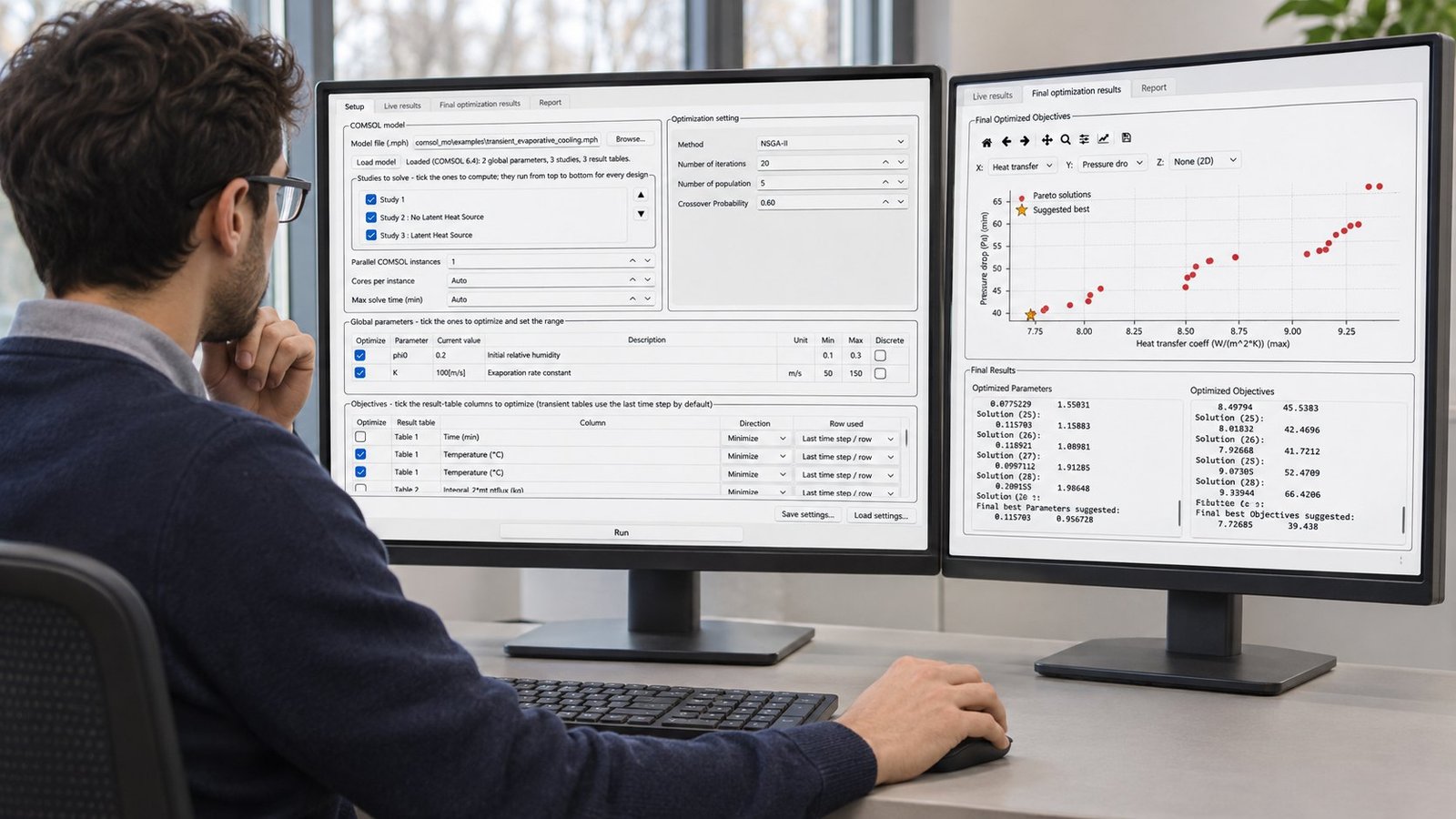
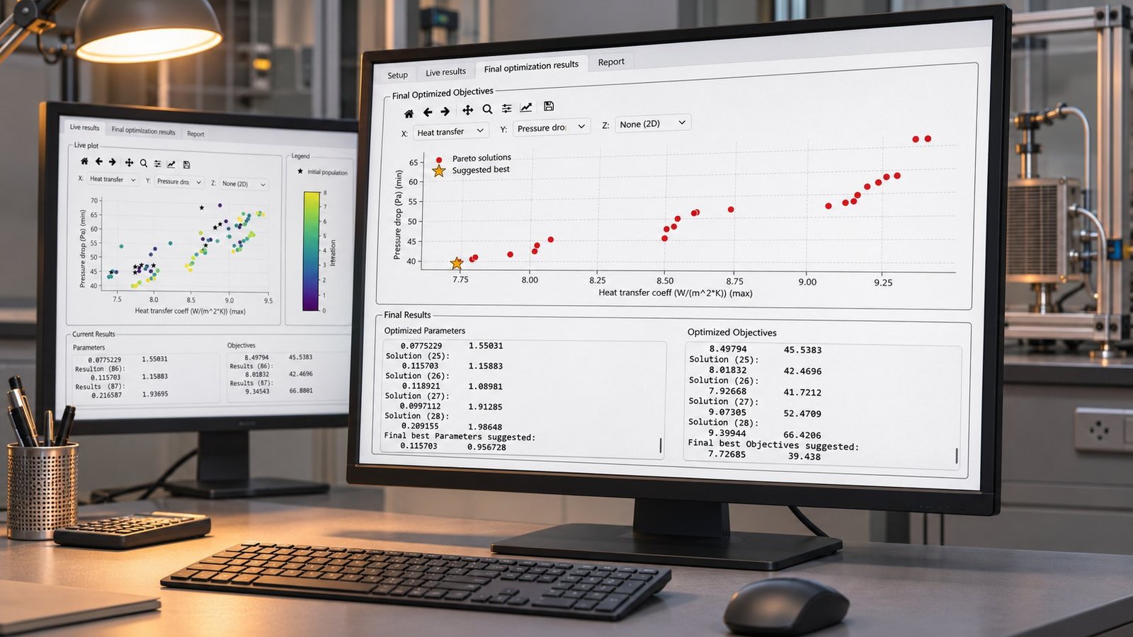
Our supplied Multi Optimization capture is a COMSOL solver baseline, not a complete surrogate accuracy claim. It identifies the exact model and optimization run, but it does not separately record neural-network training time, surrogate inference time, MAE or RMSE, or the final prediction residual after a full-solver rerun.
| Measurement | Captured first-hand value | Interpretation |
|---|---|---|
| Solver and version | COMSOL 6.4 | The loaded model reports COMSOL 6.4. |
| Physics and studies | Transient evaporative cooling; 3 studies | The setup includes Study 1, No Latent Heat Source, and Latent Heat Source. |
| Inputs and units | 2 global parameters: phi0, dimensionless, range 0.1–0.3; K, m/s, range 50–150 | The captured bounds are suitable for a bounded comparison. |
| Sample and worker count | 28 reported solutions; 1 parallel COMSOL instance; cores Auto | The report confirms a small single-worker run. |
| Wall-clock run time | 0.6418 seconds | This is the measured complete optimization time in the report. |
| Training and inference time | Not separately instrumented | Do not invent a split from the total run time. |
| Engineering error | MAE/RMSE and final rerun residual not reported | The report shows objectives, not surrogate residuals. |
| Best displayed objectives | 7.72685 and 39.438 | These are optimization results, not validation-error measurements. |
That measurement boundary is useful. Before publishing a neural network versus Kriging result from this COMSOL model, add timestamps around model fitting and batch inference, store predicted and full-solver responses for the 28 designs, and rerun the suggested best design. Then report MAE or RMSE in °C, Pa, W, or the actual response units.
See also: surrogate model comsol
When does a surrogate fail in practice?
The most useful failure cases have a trigger you can test. Solver non-convergence, unsupported categorical inputs, and extrapolation beyond the training bounds are more actionable than a generic warning about model risk.
- Solver non-convergence: remove failed designs from neither split silently. Record the trigger, constraint state, and whether the surrogate learns a feasible region.
- String variables: HEEDS 2604 cannot train its Neural Network Builder on string variables. Use a defensible numeric encoding or exclude the variable and document the limitation.
- Extrapolation: reject optimizer candidates outside the original bounds. A low interpolation error says nothing about predictions beyond those bounds.
- Unequal response scales: normalize during fitting, but report the final error in engineering units so a pressure error is not hidden by a larger temperature response.
- Sparse high-dimensional data: expand the design set before concluding that Kriging failed. A model may be accurate only where the sample density supports it.
If you are building a CFD study, the next useful reference is free cfd software for planning the sweep and cfd software for checking coolant-quality assumptions. For datacenter work, pair the training bounds with a data center cooling load rule of thumb before you extrapolate to a new operating condition.
See also: Data Center Cooling System Companies: Buyer Matrix
FAQ: neural network vs kriging
Is Kriging more accurate than a neural network?
Not always. Volupe reported lower validation error and a better Schwefel result for Kriging, but the neural network performed better on the heatsink case.
How many samples does a neural network need?
There is no reliable universal count. Use a fixed validation split, monitor error in engineering units, and add designs until the error stabilizes across the bounded space.
Should you optimize directly on a surrogate?
Use the surrogate to reduce expensive evaluations, then rerun the selected design in the full solver. Reject the result if the solver residual, constraints, or convergence behavior fails.
Conclusion
Neural network vs kriging is an engineering test, not a permanent ranking. Keep the data, bounds, validation split, and optimization budget identical. Use the HEEDS benchmark as a warning against universal claims, and use your COMSOL measurements to expose missing timing and error data. For a workflow built around parallel multi-objective optimization, review Multi Optimization parallel optimization software.