
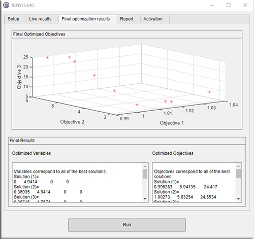
Multi-objective optimization is the process of finding the set of best possible trade-offs between two or more competing goals — for example, minimizing a building’s energy consumption while also minimizing the cost of the equipment that achieves it. Instead of one “best” answer, it produces a Pareto front: the collection of designs where improving one objective necessarily worsens another.
Why isn’t there a single best design?
Because real objectives conflict. A larger solar collector field harvests more energy but costs more. A higher chilled-water setpoint saves chiller energy but risks IT equipment temperatures. Any design that cannot be improved in one objective without sacrificing another is called non-dominated, and the set of all non-dominated designs is the Pareto front. The engineer’s job shifts from “find the optimum” to “choose a point on the front” — which is a business decision, informed by engineering.
How do algorithms like NSGA-II actually find the front?
Most practical multi-objective algorithms are evolutionary. NSGA-II — the most cited of them, published by Deb et al. in 2002 — maintains a population of candidate designs, simulates each one, ranks them by non-domination and diversity, and breeds the best to form the next generation. Over tens of generations the population converges onto the Pareto front. Particle-swarm variants like MOPSO move a swarm of designs through the search space instead of breeding them, and decomposition methods like MOEA/D split the multi-objective problem into many single-objective sub-problems. In practice, no single algorithm wins everywhere — which is why serious tools offer several.
What does this cost in simulation time?
A typical study runs 50–100 designs per generation for 20–100 generations — thousands of simulations. If one TRNSYS or COMSOL run takes five minutes, a sequential study takes days. This is why parallel evaluation matters more than algorithm choice for wall-clock time: evaluating a generation of designs across 8 CPU cores cuts the study from days to hours. Our TRNSYS MO, EES MO, and COMSOL MO tools all evaluate whole generations in parallel for exactly this reason.
How many objectives can you optimize at once?
Two or three objectives are the sweet spot for human decision-making, because the front is a curve or a surface you can plot. Beyond that, “many-objective” algorithms (NSGA-III, RVEA) use reference directions to keep the population spread out in high-dimensional objective space. Modern tools support far more — up to 99 simultaneous objectives in our applications — but the harder problem becomes visualizing and choosing among the results, which is where parallel-coordinates plots and suggested-best heuristics help.
Where do engineers use it?
- Solar thermal and building energy: collector area vs auxiliary energy vs cost (TRNSYS)
- Thermodynamic cycles: COP vs heat-exchanger size in refrigeration and heat pumps (EES)
- Multiphysics design: pressure drop vs heat transfer in heat sinks and exchangers (COMSOL)
- Data centers: PUE vs water use vs capital cost across cooling technologies
If you already have a working simulation model, you already have everything a multi-objective study needs — the optimizer supplies the rest.